plotGrouper

by John D. Gagnon
University of California, San Francisco

Table of Contents

Overview
Installation
Usage
Session info
License

Overview

A shiny app-based GUI wrapper for ggplot2 with built-in statistical analysis. Import data from file and use dropdown menus and checkboxes to specify the plotting variables, graph type, and look of your plots. Once created, plots can be saved independently or stored in a report that can be saved as a pdf. If new data are added to the file, the report can be refreshed to include new data. Statistical tests can be selected and added to the graphs.

Analysis of flow cytometry data is especially integrated with plotGrouper. Count data can be transformed to return the absolute number of cells in a sample (this feature requires inclusion of the number of beads per sample and information about any dilution performed).

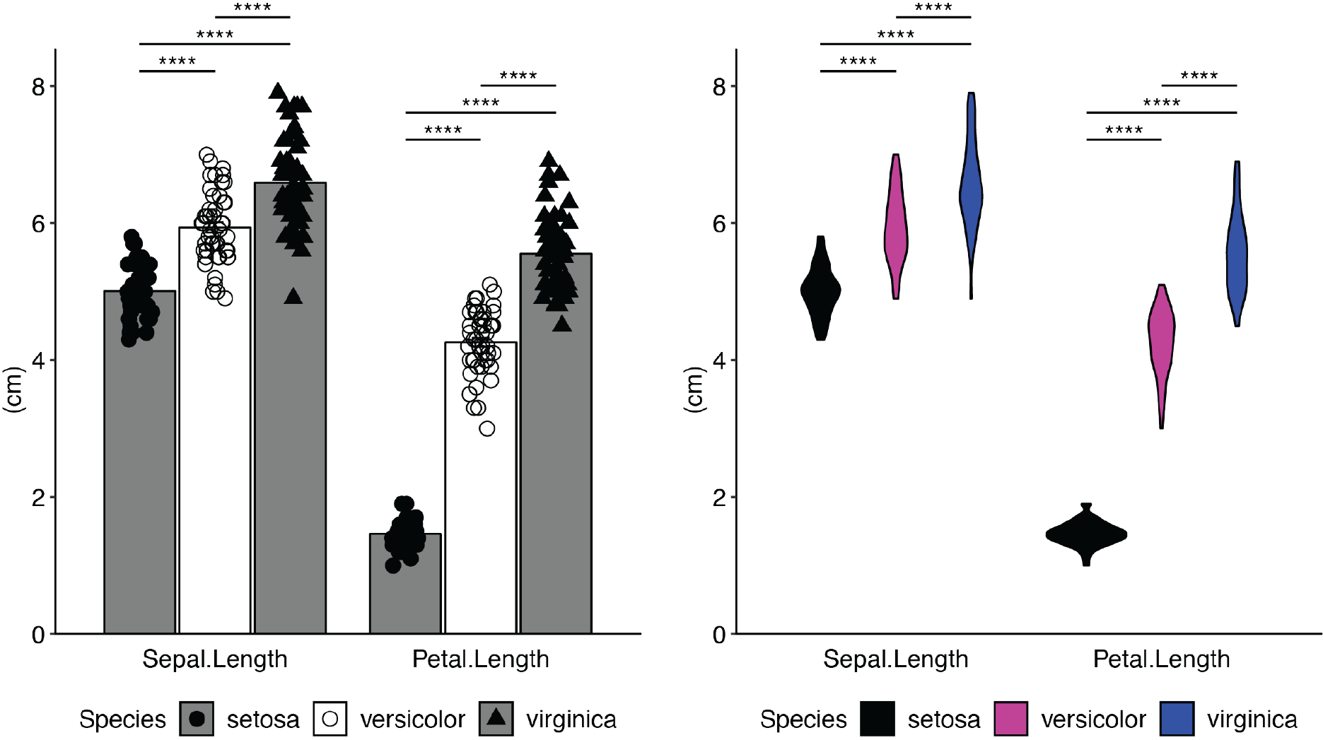
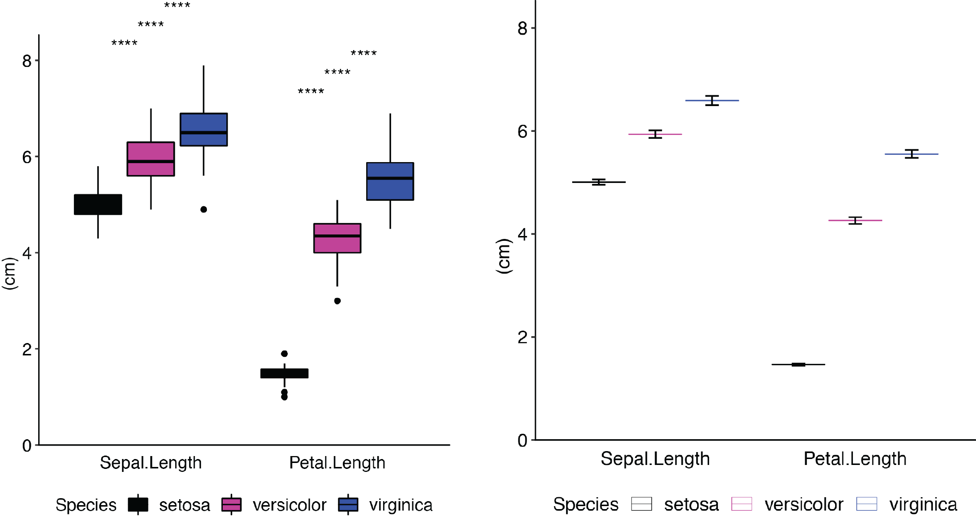
Examples of some of the types of plots you can create:

Installation

• If you do not already have R installed, or your version is out of date, download and install the latest version.

  • Optionally, install the latest version of RStudio Desktop.

• Download the package from Bioconductor.

if (!requireNamespace("BiocManager", quietly = TRUE))
  install.packages("BiocManager")
  BiocManager::install("plotGrouper")

• Or install the development version of the package from Bioconductor:

'Bioconductor'
BiocManager::install("plotGrouper", version = "devel")

• Or GitHub:

BiocManager::install("jdgagnon/plotGrouper")

Usage

Load the package into the R session.

library(plotGrouper)

To initialize the shiny app, paste the following code in your R console and run it.

plotGrouper()

Once the web app opens, you can access the iris dataset by clicking the iris button to learn how to use the app. After the iris data loads, the selection windows will be automatically populated and a graph should be displayed.
The Raw Data tab displays the structure of the data loaded. Your file should be organized in the following way:

Unique identifier	Comparisons	Variables
Sample	Species	Sepal.Length
setosa_1	setosa	5.1
setosa_2	setosa	4.9
versicolor_1	versicolor	7
versicolor_2	versicolor	6.4
virginica_1	virginica	6.3
virginica_2	virginica	5.8
etc…	etc…	etc…

These columns can be titled anything you want but values in the columns are important.

• The Unique identifier column should contain only unique values that identify each individual sample (e.g., Sample within iris Raw Data).

• The Comparisons column should contain replicated values that identify each individual as belonging to a group (e.g., Species within iris Raw Data).

• The Variables column(s) should created for each variable you wish to plot. The values in these columns must be numeric (e.g., Sepal.Length, Sepal.Width, Petal.Length, Petal.Width within iris Raw Data)

After importing a data file, a Sheet column will be created and populated with the sheet name(s) from the file if it came from an excel spreadsheet or the file name if it came from a csv or tsv file.

• The Variables to plot selection window is used to choose which variable(s) to plot (e.g., Sepal.Width from the iris data). If multiple are selected, they will be grouped according to the Independent variable selected.

• The Comparisons selection window is used to choose which column contains the information that identifies which condition each sample belongs to (e.g., the Species column within the iris data).

• The Independent variable selection window is used to select how the plots should be grouped. If variable is selected (the default), the plots will be grouped by the values in Variables to plot.

• Use the Shapes selector to change the shape of the points for each comparison variable.

• Use the Colors selector to change the point colors for each comparison variable.

• Use the Fills selector to change the fill color for the other geoms being plotted for each comparison variable.

To prevent the Shapes, Colors, or Fills from reverting to their defaults, click the Lock checkboxes.

Individual plots can be saved by clicking Save on the Plot tab or multiple plots may be arranged on a single page by clicking Add plot to report. Clicking this button will send the current plot to the Report tab and assign it a number in the Report plot # dropdown menu. To revisit a plot stored in the Report tab, select the plot you wish to restore and click Load plot from report. Changes can be made to this plot and then updated in the Report by clicking Update plot in report.

• The statistics calculated for the current plot being displayed in the Plot tab are stored in the Statistics tab. These can be saved by clicking the Download button on the Statistics tab.

• The Plot Data tab contains the reorganized subset of data being plotted.

• The Raw Data tab displays the dataframe that was created upon import of the file along with the automatically created Sheet column.

Session info

Here is the output of sessionInfo() on the system on which this package was developed:

sessionInfo()
#> R version 3.5.1 (2018-07-02)
#> Platform: x86_64-apple-darwin17.6.0 (64-bit)
#> Running under: macOS High Sierra 10.13.6
#> 
#> Matrix products: default
#> BLAS: /System/Library/Frameworks/Accelerate.framework/Versions/A/Frameworks/vecLib.framework/Versions/A/libBLAS.dylib
#> LAPACK: /System/Library/Frameworks/Accelerate.framework/Versions/A/Frameworks/vecLib.framework/Versions/A/libLAPACK.dylib
#> 
#> locale:
#> [1] en_US.UTF-8/en_US.UTF-8/en_US.UTF-8/C/en_US.UTF-8/en_US.UTF-8
#> 
#> attached base packages:
#> [1] stats     graphics  grDevices utils     datasets  methods   base     
#> 
#> loaded via a namespace (and not attached):
#>  [1] compiler_3.5.1  backports_1.1.2 magrittr_1.5    rprojroot_1.3-2
#>  [5] tools_3.5.1     htmltools_0.3.6 yaml_2.2.0      Rcpp_0.12.19   
#>  [9] stringi_1.2.4   rmarkdown_1.10  highr_0.7       knitr_1.20     
#> [13] stringr_1.3.1   digest_0.6.18   evaluate_0.12

License

GNU GPL-3.0-or-later